PART 2: FINDING MAPS IN ALBUM COVER ART USING AI
In Part 1 of Finding Maps in Album Cover Art using AI, I shared a holiday project where I hoped AI would fast-track the process of finding album covers with maps on them. After some digging around I chose ChatGPT’s CLIP model as a starting point to kick off the search. Here is what I found.
Natural Language Prompts
CLIP relies a set of natural language prompts known as ‘labels’ as inputs to pair with a mathematical pixel signature of a map. So the first task was to come up with a set of labels which would help CLIP determine if a cover included a map or not. I took a pass at listing out a bunch of labels based on my knowledge of what maps I had seen on album covers over the last decade (see samples below).
map_labels = [
    # General map representations
    "a cartographic map showing geography and political borders",
    "a detailed world map with labeled countries and oceans",
    "a regional map showing cities, roads, and borders",
    "a simplified map diagram for reference",
    "a labeled map with place names and symbols",

    # Topographic & physical maps
    "a topographic map with terrain contour lines",
    "a shaded relief map showing elevation and landforms",

...
not_map_labels = [
"a colorful hand-drawn illustration of a person or character",
"painterly artwork with visible brushstrokes and paper texture",
"a drawing of an animal in a natural setting",
"a photograph of a plant, garden, or flowers",
"a photo centered in a frame with a wide border",
"a photograph of nature with organic textures and leaves",
"a close-up photo of vegetation or a potted plant",
"abstract geometric line art with no geography",
"a portrait photo of a musician",
...I included a bunch more ‘map_labels’ around ‘Navigation & Transportation’, ‘Thematic & data maps’, ‘GIS & technical maps’, ‘Historical & vintage’, ‘Artistic & stylised’, ‘Globes & 3D’ and ‘World maps’.
For comparisons sake, I uploaded the 415 album cover maps to Gemini’s File API for Gemini 2.5 Flash to generate a set a labels (see below).
map_labels = [
    "geographical map", "topographic map", "street map", "atlas page",
    "nautical chart", "map grid lines", "landmass outlines", "world map",
    "folded paper map", "vintage cartography", "satellite imagery map"
]

not_map_labels = [
    "a close-up portrait of a person's face",
    "the circular center label of a vinyl record",
    "a person standing in front of a camera",
    "purely abstract geometric art",
    "a movie poster with large text and actors",
    "landscape photography without any map lines",
    "a blank wall with text typography",
    "a photo of a musician or band"
]
Not knowing how many labels Gemini would generate I set a max limit of 15 'map_labels' and 15 'not_map_labels‘. You will notice that Gemini provided a set of labels that were far more succinct than mine, and because of the cap there were naturally far fewer.
Map Scoring
It was important to consider how I wanted CLIP to use the labels to determine whether an album cover had a map on it or not.
I decided to start with an Additive scoring approach. This method was chosen because it prioritised recall over precision. The system effectively looks at each image in the collection and determines a single probability for each of the 'map_labels'. It adds together the confidence scores for every label in the list, and if the summed probability score is greater than the threshold (see below), the album cover is tagged ‘is_map’. This method ensured a high recall because if CLIP isn’t 100% sure about one specific type of map label, if it sees just a little bit of several different map types, they stack up into a much higher total score. In this additive approach, the 'not_map_labels‘ are really only being used for diagnostics, i.e. to see which labels were contributing to the ‘false positives’. The script identifies the single label with the highest ‘weight’ out of the entire list (both map and not-map) and reports it as the primary visual trigger. The key drawback with this approach is that it doesn’t allow for a veto from the 'not_map_labels‘.
Setting the Threshold
CLIP determines how confident it is that a map exists on an album cover based off of using the 'map_labels' and paring them to what it thinks the digital signature of a map is. Since we wanted a binary output ‘is_map’ / ‘is_not_map’ I set a threshold score for it to make the determination. I thought that if CLIP was 80% confident it was a map then tag it as so. This strict criteria would hopefully ensure that the ‘is_map’ classification is pure and contains zero covers that didn’t contain maps. By using is_map = “YES” if score > 0.80 else “no” the following results were obtained.
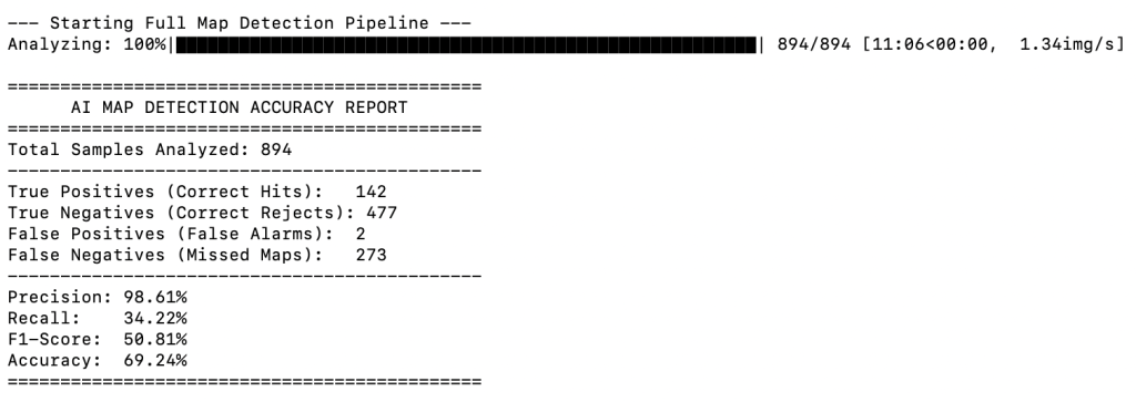
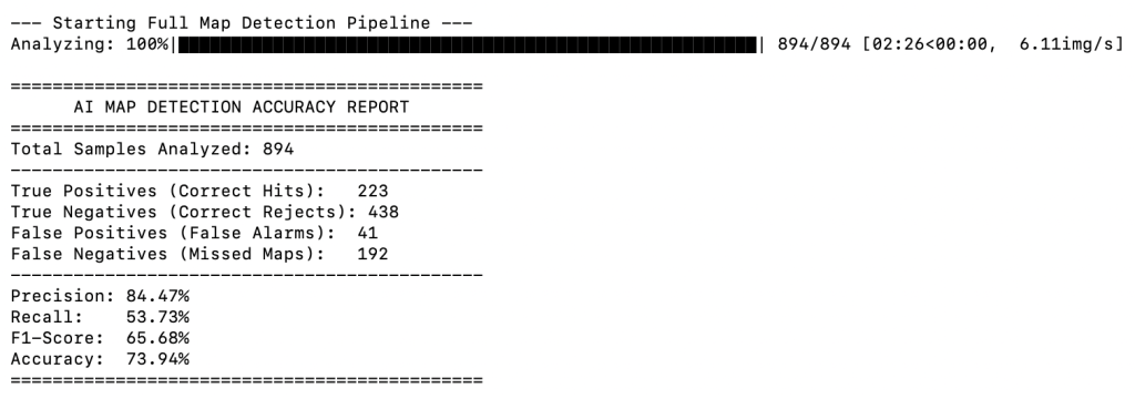
The results of using CLIP with my ‘definitive’ list of map labels and a threshold of > 0.80:
The results of using CLIP with my Gemini’s list of map labels and a threshold of > 0.80:
The script also created a new folder in my working directory called ‘detected_maps’ so I could add/delete to it as part of the post-processing validation.
What Do the Results Show?
The first thing that stands out in the reports is the processing time. A fewer number of map labels meant CLIP was left with fewer decisions to make and saw run time drop from just over 11 mins (using my labels) to ~2.5 mins (using Gemini’s labels). In this scenario the time difference is irrelevant, but for larger datasets it may become a factor.
The Gemini labels also resulted in a higher recall (223 / 142), which is a positive, however it showed up a higher number of ‘false positives’ (42 / 2). My more detailed labels effectively set a high precision, but not a very high recall, whereas the less detailed Gemini labels cast a more general net resulting in lower precision but a higher recall. Given that high recall was one of my primary goals for the project I continued to pursue improving the performance of the model using Gemini’s labels.
When I lowered the threshold to 0.50 using the Gemini labels I naturally saw an uptake in ‘true positives’, but also a bounce in ‘false positives’ (see below).

As I lowered the threshold even further to 0.10 the uptake in ‘true positives’ continued, but the ‘false positives’ also continued to grow.
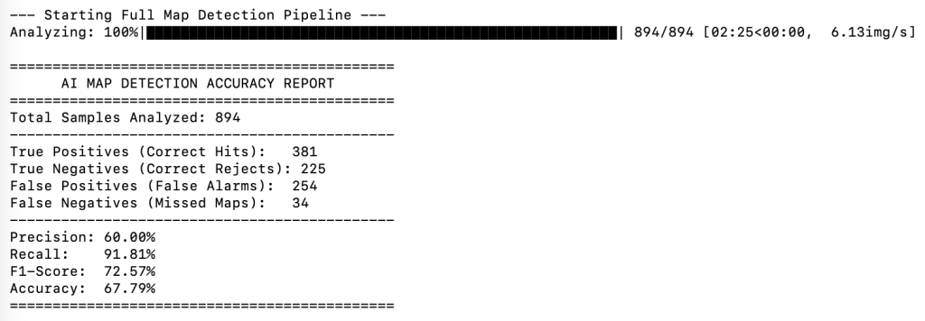
It was quickly becoming clear that I was going to have to accept a high number of ‘false positives’ if I wanted a high recall. I had to consider if it was going to be easier to bulk search and delete 254 covers that were incorrectly classified in the ‘is_maps’ folder, as opposed to trying to wade through 259 ‘is_not_map’ covers to find the 34 missed maps?
How Were the Results Validated?
The results were validated against a ground truth csv file which contained the file names of every album cover in the dataset that I had verified as having a map (as a result of creating the book). The model would therefore firstly perform its analysis and compare its results with the curated CSV file. This allowed me to see in human readable terms how well the AI’s predictions were performing.
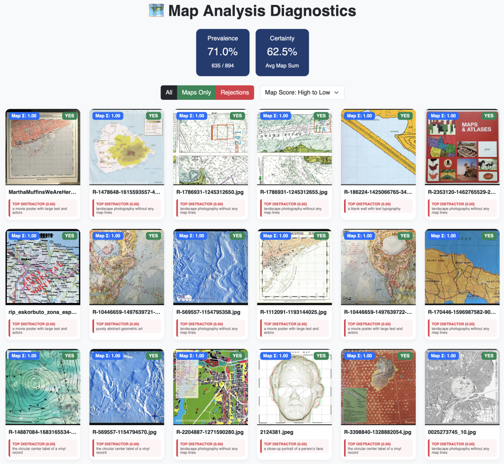
Visualising the Results
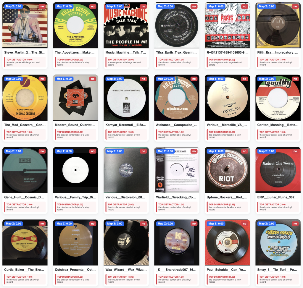
As part of the validation phase, and in order to better visualise the results (I am a visual person after all), I had Gemini write a short script which created a custom web-based dashboard that allowed me to see all of the album covers and their summed map score, as well as the top contributing 'not_map_labels‘ (top distractor). The dashboard also reported the prevalence of album covers that were tagged as having a map on them. It also reported the certainty of the model (the mean of the summed map probabilities). In the first screenshot below you can see a mediocre level of certainty being reported. This is because CLIP is often unsure about its classification of a map, but because the summed score crossed the 0.10 threshold CLIP tags it as a map. As I played around with increasing the threshold, the certainty naturally increased, however, the prevalence would drop because CLIP was no longer given a wide net to catch the artistic maps. This dashboard was incredibly useful in visually inspecting how AI was ‘seeing’ each album cover.
A Closer Inspection of What’s Happening
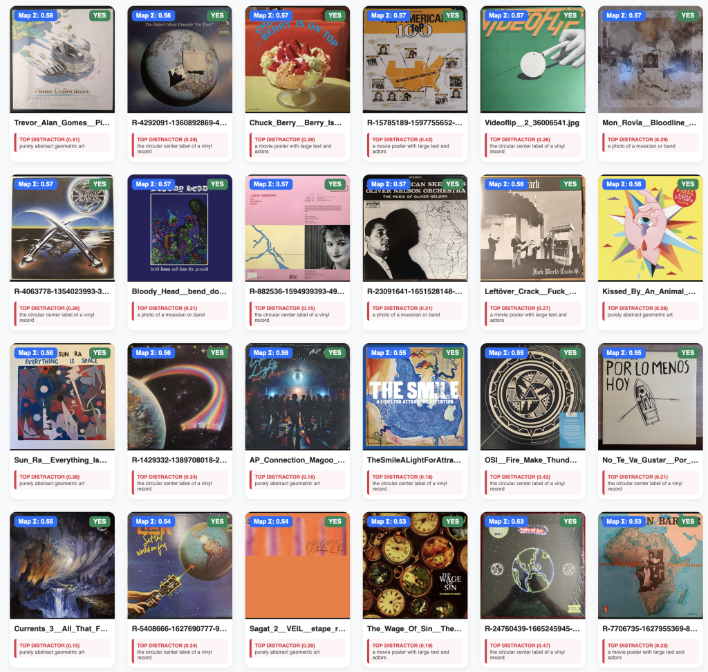
By visually inspecting the results in the dashboard I could see that sometimes CLIP’s paring of the 'map_labels‘ with the mathematical signature of other textures was causing it to incorrectly assign ‘is_map’ to covers that did not actually contain a map.
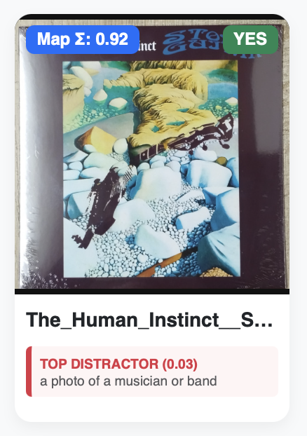
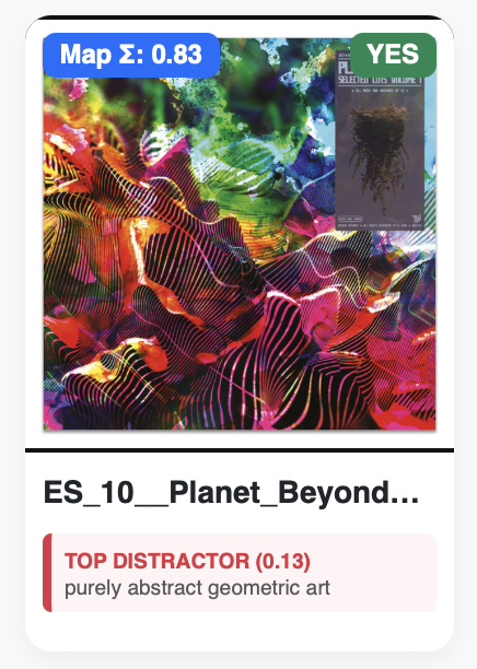
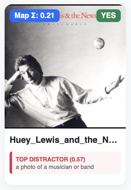
For example: The Human Instinct’s Stone Guitar cover features a broken guitar washed up on a shoreline that is depicted by an arrangement of cyan-white coloured stones. CLIP has potentially confused the signature of these textures with topographic and geographic landforms. You will see that CLIP wasn’t able to confidently label it any of the 'non_map_labels (0.03). The cover of Planet Beyond’s Selected Cuts Vol 1 features psychedelic abstract art, which CLIP may again be getting confused with the contours from a topographic map. It also assign it as ‘purely abstract geometric art’, but interestingly with not a lot of confidence (0.13). The Hewy Lewis cover is perhaps the most interesting. This cover features Hewy holding his hand out to catch a very small globe. CLIP has presumably predicted, with 0.21 confidence that this cover has a ‘world map’ on it. With 0.51 confidence CLIP determined that this cover featured ‘a photo of a musician or band’. Due to the way the Additive scoring method works, the ‘is_map’ determination wins out because it scored higher than the threshold of 0.10.
This is Part 2 of a 3-part series. In Part 3, I switch to another scoring method and also make an attempt to summarise this out-of-control holiday project!