PART 3: FINDING MAPS IN ALBUM COVER ART USING AI

In Part 2 of Finding Maps in Album Cover Art using AI, I shared the results of ChatGPT’s CLIP to fast-track the process of finding album covers with maps on them. Whilst the result were promising, I was keen to push the model further to see if I could reduce the ‘false positives’ while maintaining a high recall rate.

A Summary of The Process So Far

• ChatGPT’s CLIP was identified as potentially a ‘good’ model for automatically detecting album covers with maps on them
• A set of natural language labels were created for CLIP to pair with mathematical signatures of ‘maps’
• An additive method of scoring was set up to prioritise recall over precision
• A low threshold was set to cast a wide net to ensure few covers with maps on them were missed
• A ground truth file was used to measure the success of the model
• A dashboard was put in place to visualise the results

The Results So Far

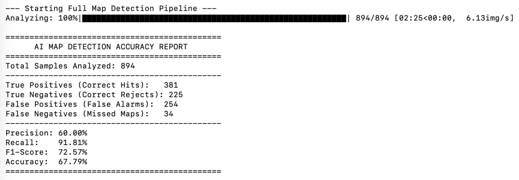
• I was achieving my goal of high recall of 91.81% (not missing maps), but in return I was getting a lot of ‘false positives’ (40%) that I would be required to sift through and delete manually.
• The additive scoring method was not utilising the 'not_map_labels', which may have been contributing to the high ‘false positive’ numbers. Basically the 'not_map_labels' were just being spectators rather than participants. I wanted to change that to see what impact it would have on the results…

Comparative Scoring

In order to move the 'not_map_labels' labels from being spectators to participants, I needed to rethink the logic of the scoring. I wanted to test what would happen when the AI had to weigh up the probability of a map against it not being a map. This would give the 'not_map_labels' probability a chance to win against the 'map_labels' probability. For example, if CLIP is 40% sure it’s a movie poster and 12% sure it’s a map, this comparative approach sees the 40% as the ‘winner’ and rejects the image as having a map on its cover.

By summing the scores of both label groups, it hopefully creates a battle between the labels. This will hopefully stop album covers from sneaking in just because they have a few grid lines or topographic textures that stack up to 0.11. It will possibly act as a filter which hopefully reduces the ‘false positives’ while maintaining high recall (fingers crossed).

Comparative Scoring Results

Additive Scoring Results

Additive v Comparative Scoring. Who wins?

Who wins depends on how you look at the results. The table below compares the results of the two methods. It shows the Additive method is really good at finding almost every map (it only missed 34, compared to the Comparative method which missed 82). However, the Comparative method is significantly better at reducing false detections (96 / 254), which means it reduces the amount of manual cleanup required.

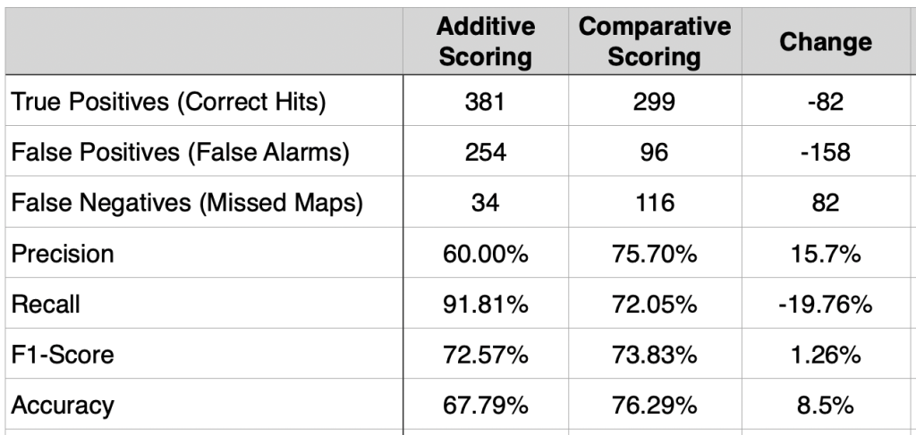
The Comparative method also increased precision by over 15%. This is positive, because it means that when the model identifies a map using comparative scoring, it is much more confident it is actually a map. The F1-Score is a machine learning metric that measures a model’s accuracy by combining its Precision and Recall into a single number. It improved only slightly in the Comparative run, suggesting that both scoring methods are performing reasonable well for this kind of dataset. According to the internet, for datasets that are artistic or ‘noisy’ (like album covers), an F1-score above 0.70 is generally considered a success.

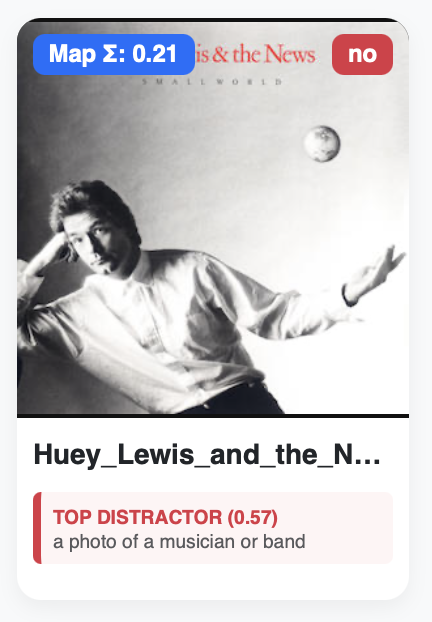
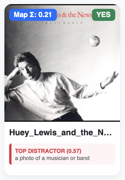
If we peek into the dashboard and compare what effect the Comparative method had on the Huey Lewis cover (that we discussed in Part 2), you will see that Comparative method performs exactly as we would expect. The 'not_map_labels' (0.57) outweighs the 'map_labels' probability (0.21), so this particular cover is tagged as not featuring a map using the Comparative method, even though it does include a very small globe floating above Huey’s hand.

Moving Forward

Where to from here? Unfortunately I don’t have access to the ‘backend’ of ChatGPT’s CLIP model to improve its understanding of what a mathematical signature of map is, so I need to stay focused on what I can control and the variables I have in front of me:

• The labels 'map_labels'and 'not_map_labels' (natural language prompts)
• The threshold
• The scoring method (additive or comparative)

Since I currently have a 91.81% recall with the additive method, perhaps I stick with it, but play around with the labels some more? I have already seen what raising the threshold achieves—see Part 2 so I will probably leave that constant for now. The number of missed maps using the Comparative method worries me a little, however perhaps this can be improved by improving the 'not_map_labels'? I also wonder how a reasoning model like Gemini 2.5 Flash might perform, as opposed to CLIP’s pattern matching?

What I do know is that this become way more than just a holiday project, and it’s time to take some time away to reset and refresh, then perhaps try some alternative combinations or models to see what direction the results move in.

Key Takeaways

For someone who spends their time colouring in maps on a daily basis (I may be slightly underselling what I do ;)), I was impressed by how quickly I was able to build a pipeline to automatically find album covers with maps on them within a massive library of music—from my laptop—while laying on a beach during holidays!

There is no doubt that without Gemini or ChatGPT to consult during the process this would not have been possible. I can’t tell you the number of questions I asked it throughout the process. If it were a technical consultant I would have racked up a bill into the tens of thousands of dollars.

It was clear that even with AI, the ideation had to be present, and the user (me) was still required to come up with a robust methodology that supported the goals of the project, and to ask the right questions at the right time (critical!). Context was also key, like setting the expectation that recall was a priority, and that to achieve a high recall it would mean wading through a bunch of false positives. This helped humanise the results.

The project also proved what I have believed for decades, that cartography and maps are a deeply complex discipline, which is misunderstood by many, including AI ;). Was I surprised by how challenged AI was at correctly identifying maps on them? Not really, because maps are complicated. They create contrast or harmony, balance or unity, beauty or intrigue, much like photography, illustration and typography, so it shouldn’t be a surprise that they share similar mathematical signatures with other textures, making it difficult for AI to distinguish between.

While the results are not ‘perfect’, it significantly reduces the burden of manual discovery by automating the initial treasure hunt through the collection. In the Additive run, the AI correctly identified 381 true maps with 91.81% recall, meaning I’m only required to manually hunt for the 34 maps the model missed. Even with the 254 false alarms, it is likely far more efficient for me to quickly delete those than to manually eyeball all 894 images in the original dataset. So for now I’m calling this a win.

Damien Saunder